Model I: Chassis

Notations & Assumptions

The notations of the parameters and variables are given as follows:

Parameters and variables

Parameters

$N_0$	The population size at the time of zero
$N_{max}$	Limitation of the population size that the environment sustain
$r$	The possible max relative growth speed
$C_i$	Proportionality factors

Variables

$N$	The current population size
$t$	Time
$P$	Product
$S$	Activated cell number

Overall Explanations of the Model

According to microbic growth process:

- Algae Growth Dynamics

Growth and Stationary
Dying(Apoptosis)
Biological stability analysis

- AGER(Product) Generation Dynamics

- Chromoprotein Production and Disease Reporting

Algae Growth Dynamics

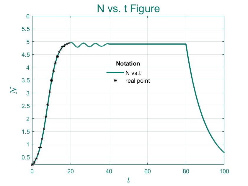
Since space and resources are limited, it is impossible to support an infinite number of algaes. When the population is too large, the birth rate decreases and the mortality rate increases due to the decrease in the average resource occupancy of algaes and the deterioration of the environment.

$N$ denotes the current population size. Let the limitation of the population size that the environment sustain be $N_{max}$. When $N < N_{max}$, the environment can still sustain the growth of population size, and as the population size keeps increasing and approaches $N_{max}$, the inhibitory effect will become more and more obvious. Then, according to the above, $N_{max}-N$ can exactly represent the number of populations that the environment can sustain,$r$ represents the possible max relative growth speed of the algaes, and $t$ represents time.

Theorem (Logistic Model)

\begin{equation} \frac{dN}{dt} = r(1-\frac{N}{N_{max}})N \end{equation}

where $N(t)|_{t=0}=N_{0}$ $\mathop{lim}\limits_{t\rightarrow\infty}N(t)=N_{max}$

Considering the solution to this OED:

$$ \begin{equation} N(t)=\frac{N_{0}N_{max}}{N_{0}+(N_{max}-N_{0})e^{-rt}} \end{equation} $$

Theorem

\begin{equation} \frac{1}{N}\frac{dN}{dt} = -D \end{equation}

where $D$ is the ratio of mortality.

Solving this ODE:

$$ \begin{equation} N(t) = N_{max}e^{-Dt} \end{equation} $$

Definition (Autonomous System)

The differential equation in the following form:

$$ \frac{dx}{dt} = f(x) $$

The differential equation in the following form: $\frac{dx}{dt} = f(x)$ is called autonomous systems, where $f(x)$ does not obviously contain a time variable. Clearly, ‘Logistic Model’ is an autonomous system.

Definition (Phase Plane)

The phase space of the autonomous system $\frac{dx}{dt} = f(x)$ is the space $\mathbb{R}^n$ with ($x_1, · · · , x_n$) as coordinates. In particular, when $n = 2$, the phase space is called the phase plane. The set of points $ \{(x_1, · · · , x_n)|x_i = x_i(t)\}$ in the space $\mathbb{R}^n$ satisfies $\frac{dx}{dt} = f(x)$, (where $i = 1,··· ,n$) called the track line of the system. The distribution of all track lines in phase space is called phase diagram.

Definition (Stability Determination:Lyapunov)

Let $x_{0}$ be the equilibrium point of $\frac{dx}{dt} = f(x)$:

$x_{0}$ is stable for any given $\varepsilon>0$,there exists a $\delta>0$ such that whenever $|x(0)-x_{0}|<\delta$, there is $|x(t)-x_{0}|<\varepsilon$,which holds for all $t$.
$x_{0}$ is asymptotically stable if it is stable and $\mathop{lim}\limits_{t\rightarrow\infty}|x(t)-x_{0}|=0$.
$x_{0}$ is unstable if the first condition above is not satisfied.

Definition

Let $x^{0}$ be the equilibrium point of the differential equation $\frac{dx}{dt} = f(x)$. If $f'(x^{0}) < 0$, then $x^{0}$ is asymptotically stable; if $f'(x^{0})>0$, then $x^{0}$ is unstable.

Proof

According to Taylor Expansion:

$$ \begin{equation*} f(x)=f(x^{0})+f'(x^{0})(x-x^{0})+o(|x-x^{0}|) \end{equation*} $$

Because $x^{0}$ is the equilibrium point, so it is obvious that $f(x^{0})=0$.
If $f'(x^{0}) < 0$, when $x < x^{0}$, then $f(x)>0$, $x$ monotonic increase; when $x>x^{0}$, then $f(x) < 0$, $x$ monotonous reduction, all above indicates that $x\rightarrow x^{0}$.
If $f'(x^{0})>0$, similar analysis process.

For Logistic Model:

\begin{equation*} f(N) = rN - \frac{rN^{2}}{N_{max}} \qquad f'(N) = r - 2\frac{rN}{N_{max}} \end{equation*}

It's obvious when $N=N_{max}$, it is asymptotically stable.

Figure: Model I Fig

AGER(Product) Generation Dynamics

Considering algaes growth and product generation as a mixed model, that is, related to both primary and secondary products(related to both cell accumulation and its growth rates).

Theorem

\begin{equation} \frac{dP}{dt} = C_{1}\frac{dN}{dt}+C_{2}N \end{equation}

where $C_1$ and $C_{2}$ are two proportionality factors.

Chromoprotein Production & Disease Reporting

Considering the rate of change of activated cells depends on the cell growth rate, the activated cell number and the amount of cell accumulation.

Theorem

\begin{equation} \frac{dS}{dt} = C_{3}N+C_{4}\frac{dN}{dt}+C_{5} S \end{equation}

where $C_{3}$, $C_{4}$ and $C_{5}$ are three proportionality factors.

Under the assumption that the production of chromoprotein is proportional to the number of activated cells, the amount of chromoprotein production can be reflected by the number of activated cells.

Model II: Hydrogel & Drug

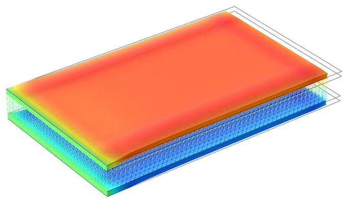
Hydrogel Phase Transition & Swelling

Theorem (Rubber Thermodynamics)

It describes the phase transition of the hydrogel and the entropy. The force $f$ that deforms the polymer network consists of two components:

\begin{equation} f = f_{e}+f_{s} =(\frac{\partial U}{\partial L})_{T,V} + T(\frac{\partial f}{\partial T})_{V,L} =(\frac{\partial U}{\partial L})_{T,V} -T(\frac{\partial S}{\partial L})_{T,V} \end{equation}

where $U$ is the internal energy, $S$ is the entropy, $L$ is the polymer length dimension, $T$ is the temperature, $V$ is the volume.

Theorem (Swelling Equilibrium)

\begin{equation} q_{m}^{5/3} \cong \frac{V_{0}}{\nu_e}\frac{(\frac{1}{2}-\chi_{1})}{\nu_1} \end{equation}

where $q_{m}^{5/3}$ is equilibrium swelling ratio, $V_0$ is volume of unswollen polymer, $\chi_{1}$ is polymer-solvent interaction coefficient, $\nu_e$ is effective number of chain segments in the polymer network, $\nu_1$ is molar volume of solvent molecules.

Hydrogel Drug Release

The model considers the phenomenon of drug diffusion as well as polymer relaxation, assuming that the drug release is a fast diffusion-controlled phenomenon and subsequently controlled by polymer chain relaxation, and the whole drug release process considers the superposition effect of two components.

Theorem (Empirical model I)

\begin{equation} M_{t} = M_{\infty,F}[1-\frac{6}{\pi^{2}}\mathop{\sum}\limits_{n=1}^{\infty}\frac{1}{n^2}exp(-n^2\frac{4\pi^2D}{d^2}t)] + M_{\infty,R}[1-exp(-k't)] \end{equation}

where $M_{t}$ is accumulated amount of drug released at moment $t$, $D$ is the diffusion coefficient of drug molecules, $d$ is the particle diameter, $M_{\infty,F}$ is the amount of accumulated drug release over an infinite period of time when no relaxation of the polymer occurs, $M_{\infty,R}$ is the total amount of drug release due to relaxation, $k'$ is the relaxation rate constant.

Theorem (Empirical model II)

\begin{equation} \frac{M_{t}}{M_{\infty}} = k'_1 t^n + k'_2 t^{2n} \end{equation}

where $k'_1$ and $k'_2$ denote the diffusion and relaxation kinetic constants, respectively.

It is preferred to use Scaling Law to determine whether this Model is suitable.

Theorem (Detailed model)

\begin{equation} F_{d}(t)=1-(\frac{r_{s}}{r_{0}})^{2}-\frac{(r_{d}^{2}-r_{s}^{2})}{f_{s}r_{0}^{2}}-\frac{2V_{poly}\rho_{poly}M_{d}}{\rho_{w}f_{s}V_{d}\rho_{d}r_{0}^{2}}\int_{r_{d}}^{r_{e}}C_{d}C_{w}rdr \end{equation}

where $F_{d}(t)$ is accumulated amount of drug released at moment $t$, $r_s$, $r_0$, $r_d$, $r_e$ denotes matrix dissolution front, original radius, diffusion front, and erosion front, respectively, $f_s$ is matrix expansion coefficient, $V_{poly}$ and $V_d$ denote matrix volume and drug volume, respectively, $\rho_{poly}$, $\rho_w$, $\rho_d$ denotes matrix density, water density, and drug density, respectively, $M_d$ is drug mass fraction, $C_d$, $C_w$ denotes drug concentration and water molecule concentration in the outermost region, respectively.

It is admitted that much of the data of the detailed model is very difficult to measure.

the Whole Process of Hydrogel Swelling & Drug Release

Kinetic processes are dynamic evolutionary processes that characterize the movement of matter from one equilibrium state to another.

Theorem

Conservation of mass:

\begin{equation} \nabla \cdot [(\phi^{w})^{2}\nabla p - f_{sw}\boldsymbol{V^{s}}] = 0 \end{equation}

Conservation of momentum:

\begin{equation} \nabla \cdot (\boldsymbol{\sigma^{s}} - p \boldsymbol{I}) = 0 \end{equation}

Pharmacodynamics:

\begin{equation} \frac{\partial c}{\partial t} + v^{w} \cdot \nabla c = \nabla \cdot (D\nabla c) \end{equation}

Constitutive equation:

\begin{equation} \boldsymbol{\sigma^{s}} = \lambda tr(\boldsymbol{\varepsilon})\boldsymbol{I} + 2\mu \boldsymbol{\varepsilon} \end{equation}

Figure: Model II Fig

Model III: Drug Absorption

Notations & Assumptions

The notations of the parameters and variables are given as follows:

Parameters and variables

Parameters

$k_i$	Proportionality factor
$R$	The total amount of drug entering the body
$V$	Volume of blood

Variables

$x(t)$	Total amount of drugs in the body at time $t$
$y(t)$	The amount of drug remaining at moment $t$
$t$	Time
$C(t)$	Drug concentration in the blood

Pharmacodynamics

The way in which drugs in biological dressings are absorbed into the body is often different from the rapid intravenous injection and constant rate intravenous drip processes.

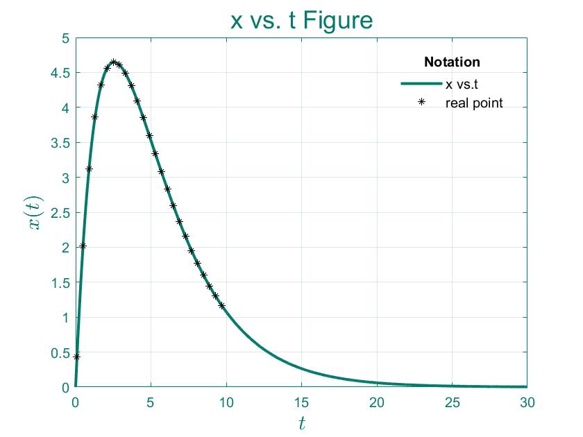
After application, the drug is generally concentrated on a certain part of the body and is gradually absorbed by the contact between its surface and the muscle. Let the rate at which the drug is absorbed be proportional to the amount of the stock drug, and note the proportionality factor as $k_{1}$. That is, if the amount of drug remaining at moment $t$ is noted as $y(t)$, then $y$ satisfies:

\begin{equation} \frac{dy}{dt} = -k_{1}y \end{equation}

where $y(0) = R$, represents the total amount of drug entering the body.

Single-compartment model of drug distribution: Assume that the drug in the body is uniformly distributed at any moment, and let the total amount of drug in moment $t$ be $x(t)$; the system is in a dynamic equilibrium, the following relationship is assumed:

\begin{equation} \frac{dx}{dt} = (\frac{dx}{dt})_{in} - (\frac{dx}{dt})_{out} \end{equation}

The rate of drug breakdown and excretion is usually considered to be proportional to the current concentration of the drug (note the proportionality factor as $k_{2}$), which is usually considered $(\frac{dx}{dt})_{out}= k_{2}x$, but the input pattern of the drug depends on the mode of administration. Considering the nature of drug delivery by application:

\begin{equation} \frac{dx}{dt} + k_{2}x = k_{1}Re^{-k_{1}t} \end{equation}

Solve the above ordinary differential equation: \begin{equation} x(t) = \frac{k_{1}R}{k_{1}-k_{2}}(e^{-k_{2}t}-e^{-k_{1}t}) \end{equation}

So the drug concentration in the blood is $C(t) = \frac{x(t)}{V}$, $V$ is the volume of blood.

Definition (Analysis)

Normally,there is always $k_{1}>k_{2}$ because the rate of input is generally greater than the rate of breakdown and excretion before the drug is absorbed, but there will be exceptions. At $k_{1}>k_{2}$ the amount of drug in the body is not very large, which in medical terms is called flip-flop; when $k_{1}=k_{2}$ , the solution of the equation can be considered as an undefined equation of type$\frac{0}{0}$, then L'Hospital's rule can be used to obtain when $k_{2}\rightarrow k_{1}$, the blood drug concentration is $C(t) = \frac{k_{1}R}{V}te^{-k_{1}t}$

Figure: Model III Fig

REFERENCES

[1] Cheng, R., Feng, F., Meng, F., Deng, C., Feijen, J., Zhong, Z., 2011. Glutathione-responsive nano-vehicles as a promising platform for targeted intracellular drug and gene delivery. Journal of controlled release 152, 2–12.
[2] Chiu, L.L., Radisic, M., 2011. Controlled release of thymosin β4 using collagen–chitosan composite hydrogels promotes epicardial cell migration and angiogenesis. Journal of Controlled Release 155, 376–385.
[3] Killion, J.A., Geever, L.M., Devine, D.M., Kennedy, J.E., Higginbotham, C.L., 2011. Mechanical properties and thermal behaviour of pegdma hydrogels for potential bone regeneration application. Journal of the mechanical behavior of biomedical materials 4, 1219–1227.
[4] Parimala, K., Sudha, M., 2012. Effect of hydrocolloids on the rheological, microscopic, mass transfer characteristics during frying and quality characteristics of puri. Food Hydrocolloids 27, 191–200.